Online Trajectory Optimization and Optimal Control via Model Predictive Control
In the previous post on iLQR, we explored a local trajectory planning algorithm that automatically provides an optimal control policy. Today, we are introducing an alternative that is more versatile and adpative in handling constraints - Model Predictive Control (MPC).

Image Credit to Shen Li, Yang Liu </p>
Unlike iLQR that plans trajectory offline in an iterative manner, MPC formulate the planning and control problem as a Quadratic Program (QP) that can be solved online. In addition, MPC naturally incorporates constraints, whereas iLQR can only enforce dynamic feasibility by forward simulation.
The core of MPC is all about making prediction. Given an objective function, MPC would plan ahead over a certain period called receding horizon, and find the optimal control actions to minimize such an objective function. The system will usually take the very first action from the prediction, make a new prediction and repeat. Making prediction at each step allows MPC to constantly account for changes and disturbances, making it robust in handling dynamic systems.
Let’s consider a nonlinear continuous dynamic system:
\[\dot{x} = f(x, u)\]To transcribe the planning and control problem into a QP, we need to first linearize and then discretize the system. Let’s first pick a point of reference about which the system is linearized. Depending on the application, such point can be either the end target or the waypoint from a sequence. Via first-order Taylor series, we obtain:
\[\begin{gathered} \dot{x} \approx f(x_d, u_d) + \nabla_{x}f(x, u)(x-x_d) + \nabla_{u}f(x, u)(u-u_d)\\ \delta \dot{x} = A \delta x + B \delta u \quad \ \\ \end{gathered}\]where the system dynamic is now described in error coordinate with respect to the reference point $(x_d, u_d)$. Then we discretize the system given a fixed time interval $dt$:
\[\delta x_{k+1} = A \delta x_k + B \delta u_k\]Once we define the objective function and the length of the receding horizon $N$, we can put everything together:
\[\begin{aligned} &\min_{x_k,\ u_k} \sum_{k=0}^N \delta x_k^T Q \delta x_k + \delta u_k^T R \delta u_k + \delta x_N^T Q_f \delta x_N \\ &\text{s.t. } \ \delta x_{0} = x_{0} - x_d\\ &\qquad \delta x_{k+1} = A \delta x_k + B \delta u_k \\ &\qquad \text{other constraints} \end{aligned}\]where the first constraint ensures that the prediction starts from the current point and the second constraint guarantess dynamic feasibility of the prediction. As mentioned before, solving this QP will us a sequence of control actions, but we generally will only take the first action and repeat the procedure at the next time step.
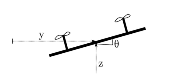
Let’s put MPC to use in a planar quadrotor.

Image Credit to Michael Posa </p>
The dynamics of the quadrotor has the following form:
\[q = \begin{bmatrix} y\\ z\\ \theta \end{bmatrix}, \qquad x = \begin{bmatrix} q \\ \dot{q} \end{bmatrix}, \qquad \ddot{q}(q,\ u) = \begin{bmatrix} - \frac{sin\theta}{m}(u_1 + u_2)\\ -g + \frac{cos\theta}{m}(u_1 + u_2)\\ \frac{a}{I}(u_1-u_2) \end{bmatrix}\]with some inertial and geometric parameters $m$, $I$, $g$, and $a$.
Say our quadrotor starts at the origin and attempts to reach and rest at a specific target, we set the receding horizon $N = 10$ with a time interval $dt = 0.1 s$. We then visualize the motion in the figure below with the red solid line representing the prediction and the black dashed line representing the actual motion.

The motion of quadrotor turns out to be rather spiral and swerving than a straight path one would expect. In reality, MPC doesn’t guarantee an “ideal” solution in all cases. A common challenge with MPC is when the receding horizon is short. In this case, the optimization does not have enough time to adjust its control actions. As a result, MPC exhibits more of a local control behavior without being able to plan ahead sufficiently.
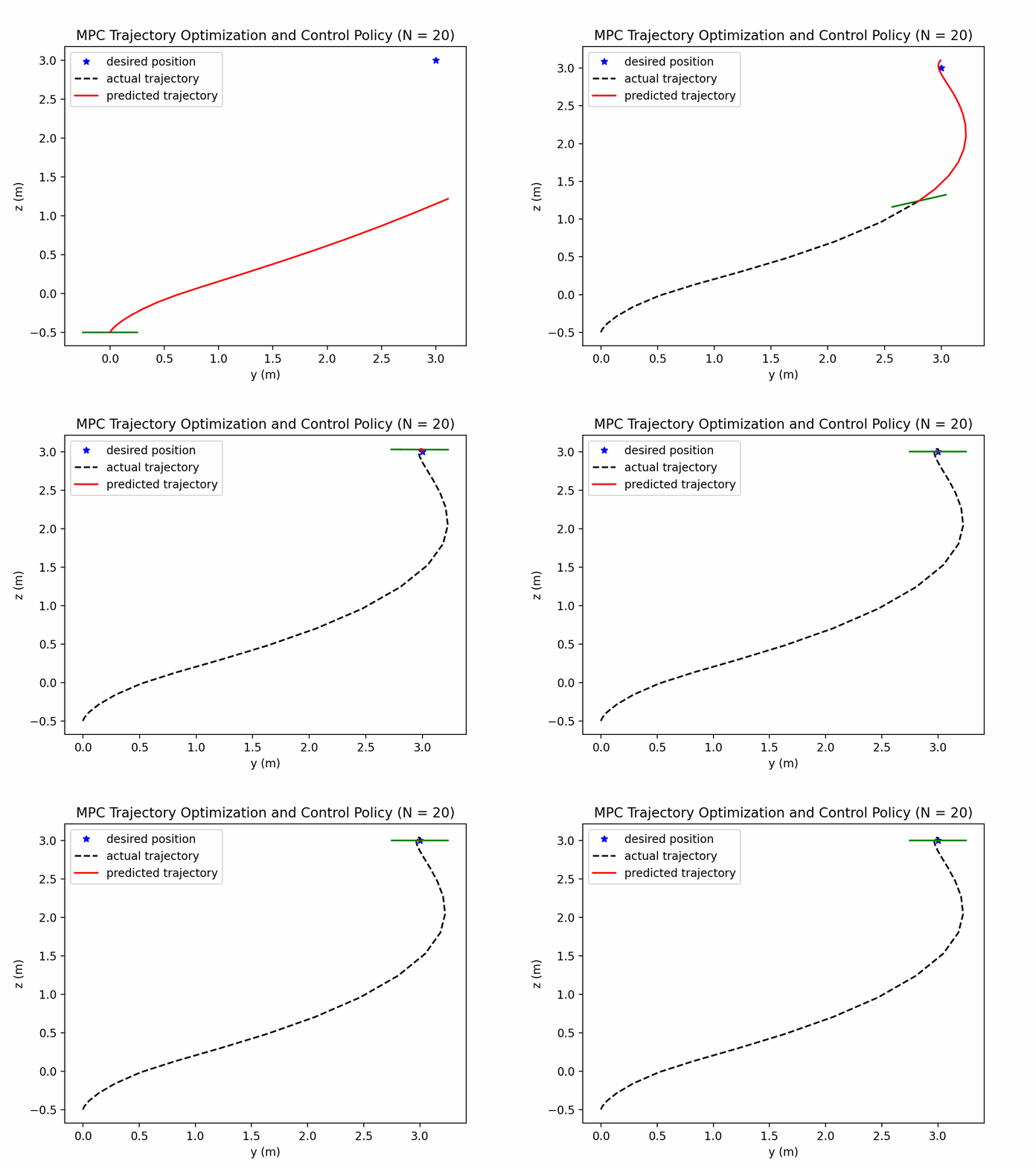
Now we extend the receding horizon by an additional 10 steps with the same time interval, i.e., $N=20$.

We observe that resulting trajectory is smoother without any spiral behaviour exhibited before. Hence, the longer prediction (red line) does help the controller to better anticipate and plan for reaching the target.
However, one should be aware that such outcome comes at the cost of increased computational complexity. It’s a trade-off between computational efficiency and the ability to handle long-term planning. Tuning the parameters of the MPC and understanding the dynamics of the system are crucial in addressing these challenges.